Introduction

Decision Tree learning is used to approximate discrete valued target functions, in which the learned function is approximated by Decision Tree. To imagine, think of decision tree as if or else rules where each if-else condition leads to certain answer at the end. You might have seen many online games which asks several question and lead to something that you would have thought at the end. A classic famous example where decision tree is used is known as Play Tennis.

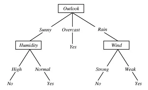
If the outlook is sunny and humidity is normal, then yes, you may play tennis.

Where should you use decision tree?

At any scenario where learning data has following traits:

The learning data has attribute value pair like in the example shown above: Wind as an attribute has two possible values – strong or weak
Target function has discreet output. Here, the target function is – should you play tennis? And the output to this discreet output – Yes and No
The training data might be missing or have error

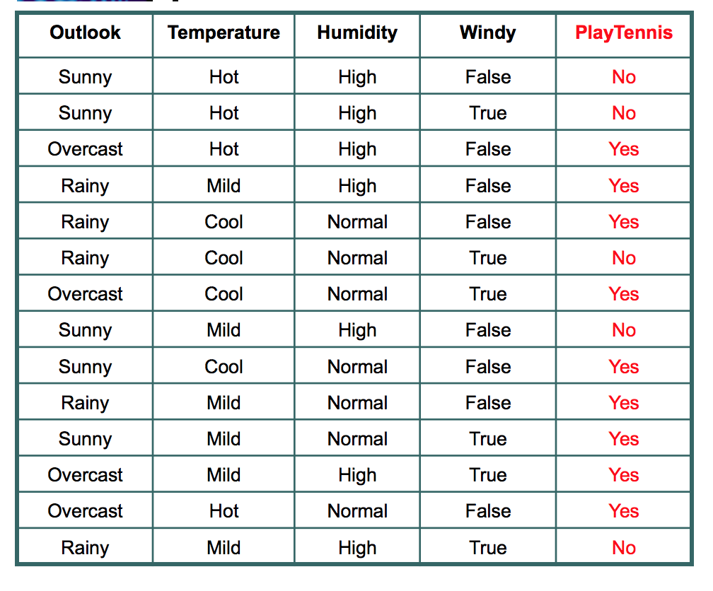
Dataset for Play Tennis

ID3 Algorithm

Although there are various decision tree learning algorithms, we will explore the Iterative Dichotomiser 3 or commonly known as ID3. ID3 was invented by Ross Quinlan.

Before we deep down further, we will discuss some key concepts:

Entropy

Entropy is a measure of randomness. In other words, its a measure of unpredictability. We will take a moment here to give entropy in case of binary event(like the coin toss, where output can be either of the two events, head or tail) a mathematical face:

Entropy = -(probability(a) * log2(probability(a))) – (probability(b) * log2(probability(b)))

where probability(a) is probability of getting head and probability(b) is probability of getting tail.

Of course this formulae can be generalised for n discreet outcome as follow:

Entropy = -p(1)*log2(p(1)) -p(2)*log2(p(2))-p(3)*log2(p(3))………………………..p(n)*log(2p(n))

Entropy is an important concept. You can find more descriptive explanation here.

Information Gain

In the decision tree shown here:

We decided to break the first decision on the basis of outlook. We could have our first decision based on humidity or wind but we chose outlook. Why?

Because making our decision on the basis of outlook reduced our randomness in the outcome(which is whether to play or not), more than what it would have been reduced in case of humidity or wind.

Let’s understand with the example here. Please refer to the play tennis dataset that is pasted above.

We have data for 14 days. We have only two outcomes :

Either we played tennis or we didn’t play.

In the given 14 days, we played tennis on 9 occasions and we did not play on 5 occasions.

Probability of playing tennis:

Number of favourable events : 9

Number of total events : 14

Probability = (Number of favourable events) / (Number of total events)

= 9/14

= 0.642

Now, we will see probability of not playing tennis.

Probability of not playing tennis:

Number of favourable events : 5

Number of total events : 14

Probability = (Number of favourable events) / (Number of total events)

=5/14

=0.357

And now entropy of outcome,

Entropy at source= -(probability(a) * log2(probability(a))) – (probability(b) * log2(probability(b)))

= -(Probability of playing tennis) * log2(Probability of playing tennis) – (Probability of not playing tennis) * log2(Probability of not playing tennis)

= -0.652 * log2(0.652) – 0.357*log2(0.357)

=0.940

So, entropy of whole system before we make our firest question is 0.940

Now, we have four features to make decision and they are:

Outlook
Temperature
Windy
Humidity

Let’s see what happens to entropy when we make our first decision on the basis of Outlook.

Outlook

If we make a decison tree divison at this level 0 based on outlook, we have three branches possible; either it will be Sunny or Overcast or it will be Raining.

Sunny : In the given data, 5 days were sunny. Among those 5 days, tennis was played on 2 days and tenis was not played on 3 days. What is the entropy here?

Probablity of playing tennis = 2/5 = 0.4

Probablity of not playing tennis = 3/5 = 0.6

Entropy when sunny = -0.4 * log2(0.4) – 0.6 * log2(0.6)

= 0.97

2. Overcast: In the given data, 4 days were overcast and tennis was played on all the four days. Let

Probablity of playing tennis = 4/4 = 1

Probablity of not playing tennis = 0/4 = 0

Entropy when overcast = 0.0

3. Rain: In the given data, 5 days were rainy. Among those 5 days, tennis was played on 3 days and tenis was not played on 2 days. What is the entropy here?

Probablity of not playing tennis = 2/5 = 0.4

Probablity of playing tennis = 3/5 = 0.6

Entropy when rainy = -0.4 * log2(0.4) – 0.6 * log2(0.6)

= 0.97

Entropy among the three branches:

Entropy among three branches = ((number of sunny days)/(total days) * (entropy when sunny)) + ((number of overcast days)/(total days) * (entropy when overcast)) + ((number of rainy days)/(total days) * (entropy when rainy))

= ((5/14) * 0.97) + ((4/14) * 0) + ((5/14) * 0.97)

= 0.69

What is the reduction is randomness due to choosing outlook as a decsion maker?

Reduction in randomness = entropy source – entropy of branches

= 0.940 – 0.69

= 0.246

This reduction in randomness is called Information Gain. Similar calculation can be done for other features.

Temperature

Information Gain = 0.029

Windy

Information Gain = 0.048

Humidity

Information Gain = 0.152

We can see that decrease in randomness, or information gain is most for Outlook. So, we choose first decision maker as Outlook.

Pseudocode

Create feature list, attribute list.

Example: Feature List : Outlook, Windy, Temperature and Humidity

Attributes for Outlook are Sunny, Overcast and Rainy.

2. Find the maximum information gain among all the features. Assign it root node.

Outlook in our example and it has three branches: Sunny, Overcast and Rainy.

3. Remove the feature assigned in root node from the feature list and again find the maximum increase in information gain for each branch. Assign the feature as child node of each brach and remove that feature from featurelist for that branch.

Sunny Branch for outlook root node has humidity as child node.

4. Repeat step 3 until you get branches with only pure leaf. In our example, either yes or no.