
Prerequisite
Python, Scikit and Panda installed in your laptop. It’s better to install conda as it has all the required libraries. Install Jupyter too. It really helps in python coding.
Panda
Panda is a popular python library to explore and manipulate data.
Scikit
Scikit is popular machine learning framework in python.
Regression
Regression is process to find relation between one variable and several dependent variable. There are many regression techniques like linear regression, simple regression ordinary least squares to name a few.
Decision Tree Regression
Suppose you have the following data with you about the number of a bathroom in a house and it’s price:
| Number of Bathroom | Price |
| 1 | 10000 |
| 2 | 10000 |
| 3 | 30000 |
You might infer from the data above that whenever number of bathrooms in house is less than three, price is 10000 else it is 30000. Same inference can be put in the following way.
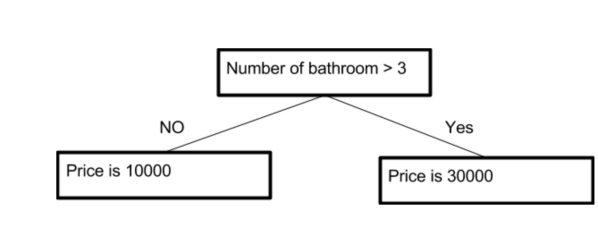
This is an example of decision tree, albeit very crude of level one. Here, we have only two leaf. So, the lack of data makes us think that if a house has 7 bathrooms, it will still have 30000 as price. Now, you can think that scikit models can go upto level 10 which will have around 1000 leaf and that model will be more accurate than this. We have used Decision Tree Regression to predict the pricing of House in Melbourne.
Dataset
Please download the dataset from here.
Example
In the example shown below, comments are added at each step. Please go through the code once and make your first ML model. This example has been done in jupyter notebook so ignore comments like #In[6]
| # coding: utf-8 | |
| # In[1]: | |
| #Pandas is the primary tool that modern data scientists use for exploring and manipulating data. Let's import it. | |
| import pandas as pd | |
| # In[6]: | |
| #let's load the housing data for melbourne | |
| data_file_path = "/Users/harshvardhan/learning_scikit/data/melb_data.csv" #replace the path with your file path | |
| #panda's read_csv method reads the csv file and loads into a data structure called data_frame | |
| #imagine data_frame as sql table | |
| melbourne_data_frame = pd.read_csv(data_file_path) | |
| #let's show first two rows of the csv/data_frame to get a feel of the data | |
| melbourne_data_frame[:2] | |
| # In[3]: | |
| #Describe method gives us 8 attributes of each column of csv: | |
| #They are 1. Count (Total valid values) 2. Mean (Average) 3. std (Standard Deviation) 4. min (Minimum in that column) | |
| #5. 25% (25th percentile) 6. 50% (50th Percentile) 7. 75% (75th Percentile) 8. Max(Maximum in that column) | |
| melbourne_data_frame.describe() | |
| # In[8]: | |
| #Selecting one column of data frame using panda | |
| price_column = melbourne_data_frame.Price | |
| #head method prints first few data of the column | |
| price_column.head() | |
| # In[10]: | |
| #Selecting more than one coulmn; store the name of coulmn in an array | |
| rooms_price_column_name = ["Rooms","Price"] | |
| rooms_price_column = melbourne_data_frame[rooms_price_column_name] | |
| #Let's verify. Shall we? Again, the head command. | |
| rooms_price_column.head() | |
| # In[11]: | |
| #Let's pick our problem statement. It's kind of simple. We need to build a model to predict price of a house. | |
| #Think of it this way. An old couple Mr. and Mrs. Waugh who owns two houses in Melbourne wants to sell one of | |
| #them. They have all the data of their house ready with them but unfortunately, they don't know the price. | |
| #So, our target is to find price and consequently we will name Price as target column. Follwing the general tradition, | |
| # where function is written as y = f(x), we will call price column as y. | |
| y = price_column | |
| # In[39]: | |
| #Now, let's talk about f(x) here. To start with, let's assume that out of several data given about the house; we think | |
| # that the price of house in melbourne depends on number of rooms, number of bathroom, landsize, building area, and | |
| #year in which it is built. we will call them predictors of price. Obviously, price depends on other factors. But | |
| #what the heck, let's get started. | |
| melbourne_price_predictors_coulmn = ['Rooms', 'Bathroom', 'Landsize', 'BuildingArea','YearBuilt'] | |
| #Going with tradition, thse are variables x of function f(x) | |
| X_raw = melbourne_data_frame[melbourne_price_predictors_coulmn] | |
| # In[40]: | |
| #What is the our input has bad values or missing values? Imputer replaces those missing values with some other value. | |
| from sklearn.preprocessing import Imputer | |
| my_imputer = Imputer() | |
| X = my_imputer.fit_transform(X_raw) | |
| # In[42]: | |
| #here, we split the given data in 2 parts. one for making model and other for validating it. | |
| #train_X is training and val_X is for validating the data. | |
| from sklearn.model_selection import train_test_split | |
| train_X, val_X, train_y, val_y = train_test_split(X, y,random_state = 0) | |
| # In[43]: | |
| #we have x and y. Where is f(x)? | |
| #so f(x) here is decision tree model. Read the blog text to find out about decision tree. scikit provides us | |
| #several models (f(x)) to predict a quantity. They are of several kinds..decision Tree, Logistic Regression, | |
| #Linear Regression. In terms of usage, it does the same work what we used to do in cartesian plane by extending | |
| #the straight line (Remember regression?) All the scikit regression models implement two methods fit() and predict() | |
| #Let's start with importing decision tree regression model | |
| from sklearn.tree import DecisionTreeRegressor | |
| # In[44]: | |
| #We will now tell regressor to give us f(x). we will give x to our regressor, f to give us f(x) | |
| #I hope i am making sense here. | |
| #let's define function f here. | |
| decision_tree_regressor = DecisionTreeRegressor() | |
| #Tell the regressor to act on predictors, x and give us a f(x). This is done by a fit method | |
| decison_tree_model = decision_tree_regressor.fit(train_X, train_y) | |
| # In[51]: | |
| #Ready to test? Let's print the second row of our data frame | |
| val_y | |
| # In[57]: | |
| #the price is 340000.0 for first validation entry,now let's give the same data to our model | |
| predicted_price = decision_tree_regressor.predict(val_X) | |
| print(predicted_price) | |
| # In[59]: | |
| #the model predicted price for the first entry as 46000 which is 12000 off the real price. | |
| #To calculate how good is our model, we are going to find mean absolute error. What is mean absolute error? | |
| # error is real_value – predicted value. mean absolute error is the mean of errors. | |
| #let's find the mean average error for our predicted prices and go home, sleep. | |
| from sklearn.metrics import mean_absolute_error | |
| print(mean_absolute_error(val_y, predicted_price)) | |
| # In[ ]: | |
| #395864.829956 is mean error value. That's a very bad mean error value. We are predicting prices too much away from the real one. Let's try to make it better | |
| #next time. | |
Find how to implement ml model in java here.
You can also see tutorial of DanB at kaggle here.
If you liked this article and would like one such blog to land in your inbox every week, consider subscribing to our newsletter: https://skillcaptain.substack.com
